Sección 6 Diagnóstico y mejora de modelos

6.1 Aspectos generales

Al comenzar un proyecto de machine learning, las primeras consideraciones deben ser:

Establecer métricas de error apropiadas para el problema, y cuál es el máximo valor de este error requerido para nuestra aplicación.
Construir un pipeline lo antes posible que vaya de datos hasta medición de calidad de los modelos. Este pipeline deberá, al menos, incluir cálculos de entradas, medición de desempeño de los modelos y cálculos de otros diagnósticos (como error de entrenamiento, convergencia de algoritmos, etc.)

En general, es difícil preveer exactamente qué va a funcionar para un problema particular, y los diagnósticos que veremos requieren de haber ajustado modelos. Nuestra primera recomendación para ir hacia un modelo de mejor desempeño es:

Es mejor y más rápido comenzar rápido, aún con un modelo simple, con entradas {} (no muy refinadas), y con los datos que tenemos a mano. De esta forma podemos aprender más rápido. Demasiado tiempo pensando, discutiendo, o diseñando qué algoritmo deberíamos usar, cómo deberíamos construir las entradas, etc. es muchas veces tiempo perdido.

Con el pipeline establecido, si el resultado no es satisfactorio, entonces tenemos que tomar decisiones para mejorar.

6.2 ¿Qué hacer cuando el desempeño no es satisfactorio?

Supongamos que tenemos un clasificador construido con regresión logística regularizada, y que cuando lo aplicamos a nuestra muestra de prueba el desempeño es malo. ¿Qué hacer?

Algunas opciones:

Conseguir más datos de entrenamiento.
Reducir el número de entradas por algún método (eliminación manual, componentes principales, etc.)
Construir más entradas utilizando distintos enfoques o fuentes de datos.
Incluir variables derivadas adicionales e interacciones.
Intentar construir una red neuronal para predecir (otro método).
Aumentar la regularización.
Disminuir la regularización.
Correr más tiempo el algoritmo de ajuste.

¿Con cuál empezar? Cada una de estas estrategias intenta arreglar distintos problemas. En lugar de intentar al azar distintas cosas, que consumen tiempo y dinero y no necesariamente nos van a llevar a mejoras, a continuación veremos diagnósticos y recetas que nos sugieren la mejor manera de usar nuestro tiempo para mejorar nuestros modelos.

Usaremos el siguiente ejemplo para ilustrar los conceptos:

Ejemplo

Nos interesa hacer una predicción de polaridad de críticas o comentarios de pelíıculas: buscamos clasificar una reseña como positiva o negativa dependiendo de su contenido. Tenemos dos grupos de reseñas separadas en positivas y negativas (estos datos fueron etiquetados por una persona).

Cada reseña está un archivo de texto, y tenemos 1000 de cada tipo:

negativos <- list.files('./datos/sentiment/neg', full.names = TRUE)
positivos <- list.files('./datos/sentiment/pos', full.names = TRUE)
head(negativos)

## [1] "./datos/sentiment/neg/cv000_29416.txt"
## [2] "./datos/sentiment/neg/cv001_19502.txt"
## [3] "./datos/sentiment/neg/cv002_17424.txt"
## [4] "./datos/sentiment/neg/cv003_12683.txt"
## [5] "./datos/sentiment/neg/cv004_12641.txt"
## [6] "./datos/sentiment/neg/cv005_29357.txt"

head(positivos)

## [1] "./datos/sentiment/pos/cv000_29590.txt"
## [2] "./datos/sentiment/pos/cv001_18431.txt"
## [3] "./datos/sentiment/pos/cv002_15918.txt"
## [4] "./datos/sentiment/pos/cv003_11664.txt"
## [5] "./datos/sentiment/pos/cv004_11636.txt"
## [6] "./datos/sentiment/pos/cv005_29443.txt"

length(negativos)

## [1] 1000

length(positivos)

## [1] 1000

read_file(negativos[1])

[1] “plot : two teen couples go to a church party , drink and then drive . get into an accident . of the guys dies , but his girlfriend continues to see him in her life , and has nightmares . ’s the deal ? the movie and " sorta " find out . . . : a mind-fuck movie for the teen generation that touches on a very cool idea , but presents it in a very bad package . is what makes this review an even harder one to write , since i generally applaud films which attempt to break the mold , mess with your head and such ( lost highway & memento ) , but there are good and bad ways of making all types of films , and these folks just didn’t snag this one correctly . seem to have taken this pretty neat concept , but executed it terribly . what are the problems with the movie ? , its main problem is that it’s simply too jumbled . starts off " normal " but then downshifts into this " fantasy " world in which you , as an audience member , have no idea what’s going on . are dreams , there are characters coming back from the dead , there are others who look like the dead , there are strange apparitions , there are disappearances , there are a looooot of chase scenes , there are tons of weird things that happen , and most of it is simply not explained . i personally don’t mind trying to unravel a film every now and then , but when all it does is give me the same clue over and over again , i get kind of fed up after a while , which is this film’s biggest problem . ’s obviously got this big secret to hide , but it seems to want to hide it completely until its final five minutes . do they make things entertaining , thrilling or even engaging , in the meantime ? really . sad part is that the arrow and i both dig on flicks like this , so we actually figured most of it out by the half-way point , so all of the strangeness after that did start to make a little bit of sense , but it still didn’t the make the film all that more entertaining . guess the bottom line with movies like this is that you should always make sure that the audience is " into it " even before they are given the secret password to enter your world of understanding . mean , showing melissa sagemiller running away from visions for about 20 minutes throughout the movie is just plain lazy ! ! , we get it . . . there people chasing her and we don’t know who they are . we really need to see it over and over again ? about giving us different scenes offering further insight into all of the strangeness going down in the movie ? , the studio took this film away from its director and chopped it up themselves , and it shows . might’ve been a pretty decent teen mind-fuck movie in here somewhere , but i guess " the suits " decided that turning it into a music video with little edge , would make more sense . actors are pretty good for the most part , although wes bentley just seemed to be playing the exact same character that he did in american beauty , only in a new neighborhood . my biggest kudos go out to sagemiller , who holds her own throughout the entire film , and actually has you feeling her character’s unraveling . , the film doesn’t stick because it doesn’t entertain , it’s confusing , it rarely excites and it feels pretty redundant for most of its runtime , despite a pretty cool ending and explanation to all of the craziness that came before it . , and by the way , this is not a horror or teen slasher flick . . . it’s packaged to look that way because someone is apparently assuming that the genre is still hot with the kids . also wrapped production two years ago and has been sitting on the shelves ever since . . . . skip ! ’s joblo coming from ? nightmare of elm street 3 ( 7/10 ) - blair witch 2 ( 7/10 ) - the crow ( 9/10 ) - the crow : salvation ( 4/10 ) - lost highway ( 10/10 ) - memento ( 10/10 ) - the others ( 9/10 ) - stir of echoes ( 8/10 ) ”

read_file(positivos[1])

[1] “films adapted from comic books have had plenty of success , whether they’re about superheroes ( batman , superman , spawn ) , or geared toward kids ( casper ) or the arthouse crowd ( ghost world ) , but there’s never really been a comic book like from hell before . starters , it was created by alan moore ( and eddie campbell ) , who brought the medium to a whole new level in the mid ‘80s with a 12-part series called the watchmen . say moore and campbell thoroughly researched the subject of jack the ripper would be like saying michael jackson is starting to look a little odd . book ( or " graphic novel , " if you will ) is over 500 pages long and includes nearly 30 more that consist of nothing but footnotes . other words , don’t dismiss this film because of its source . you can get past the whole comic book thing , you might find another stumbling block in from hell’s directors , albert and allen hughes . the hughes brothers to direct this seems almost as ludicrous as casting carrot top in , well , anything , but riddle me this : who better to direct a film that’s set in the ghetto and features really violent street crime than the mad geniuses behind menace ii society ? ghetto in question is , of course , whitechapel in 1888 london’s east end . ’s a filthy , sooty place where the whores ( called " unfortunates " ) are starting to get a little nervous about this mysterious psychopath who has been carving through their profession with surgical precision . the first stiff turns up , copper peter godley ( robbie coltrane , the world is not enough ) calls in inspector frederick abberline ( johnny depp , blow ) to crack the case . , a widower , has prophetic dreams he unsuccessfully tries to quell with copious amounts of absinthe and opium . arriving in whitechapel , he befriends an unfortunate named mary kelly ( heather graham , say it isn’t so ) and proceeds to investigate the horribly gruesome crimes that even the police surgeon can’t stomach . don’t think anyone needs to be briefed on jack the ripper , so i won’t go into the particulars here , other than to say moore and campbell have a unique and interesting theory about both the identity of the killer and the reasons he chooses to slay . the comic , they don’t bother cloaking the identity of the ripper , but screenwriters terry hayes ( vertical limit ) and rafael yglesias ( les mis ? rables ) do a good job of keeping him hidden from viewers until the very end . ’s funny to watch the locals blindly point the finger of blame at jews and indians because , after all , an englishman could never be capable of committing such ghastly acts . from hell’s ending had me whistling the stonecutters song from the simpsons for days ( " who holds back the electric car/who made steve guttenberg a star ? " ) . ’t worry - it’ll all make sense when you see it . onto from hell’s appearance : it’s certainly dark and bleak enough , and it’s surprising to see how much more it looks like a tim burton film than planet of the apes did ( at times , it seems like sleepy hollow 2 ) . print i saw wasn’t completely finished ( both color and music had not been finalized , so no comments about marilyn manson ) , but cinematographer peter deming ( don’t say a word ) ably captures the dreariness of victorian-era london and helped make the flashy killing scenes remind me of the crazy flashbacks in twin peaks , even though the violence in the film pales in comparison to that in the black-and-white comic . winner martin childs’ ( shakespeare in love ) production design turns the original prague surroundings into one creepy place . the acting in from hell is solid , with the dreamy depp turning in a typically strong performance and deftly handling a british accent . holm ( joe gould’s secret ) and richardson ( 102 dalmatians ) log in great supporting roles , but the big surprise here is graham . cringed the first time she opened her mouth , imagining her attempt at an irish accent , but it actually wasn’t half bad . film , however , is all good . 2 : 00 - r for strong violence/gore , sexuality , language and drug content ”

Consideremos primero la métrica de error, que depende de nuestra aplicación. En este caso, quisiéramos hacer dar una calificación a cada película basada en el % de reseñas positivas que tiene. Supongamos que se ha decidido que necesitamos al menos una tasa de correctos de 90% para que el score sea confiable (cómo calcularías algo así?).
Ahora necesitamos construir un pipeline para obtener las primeras predicciones. Tenemos que pensar qué entradas podríamos construir.

6.3 Pipeline de procesamiento

Empezamos por construir funciones para leer datos (ver script). Construimos un data frame:

source('./scripts/funciones_sentiment.R')
df <- prep_df('./datos/sentiment/') %>% unnest(texto)
nrow(df)

[1] 2000

str_sub(df$texto[1], 1, 200)

[1] “Review films adapted from comic books have had plenty of success , whether they’re about superheroes ( batman , superman , spawn ) , or geared toward kids ( casper ) or the arthouse crowd ( ghost wor”

Ahora separamos una muestra de prueba (y una de entrenamiento más chica para simular después el proceso de recoger más datos):

set.seed(94512)
df$muestra <- sample(c('entrena', 'prueba'), 2000, prob = c(0.8, 0.2),
                     replace = TRUE)
table(df$muestra)

## 
## entrena  prueba 
##    1575     425

df_ent <- df %>% filter(muestra == 'entrena')
df_pr <- df %>% filter(muestra == 'prueba')
df_ent <- sample_n(df_ent, nrow(df_ent)) #permutamos al azar
df_ent_grande <- df_ent
df_ent <- df_ent %>% sample_n(700)

Intentemos algo simple para empezar: consideramos qué palabras contiene cada reseña, e intentamos clasificar en base esas palabras. Así que en primer lugar dividimos cada texto en tokens (pueden ser palabras, o sucesiones de caracteres o de palabras de tamaño fijo (n-gramas), oraciones, etc.). En este caso, usamos el paquete tidytext. La función unnest_tokens elimina signos de puntuación, convierte todo a minúsculas, y separa las palabras:

Vamos a calcular los tokens y ordernarlos por frecuencia. Empezamos calculando nuestro vocabulario. Supongamos que usamos las 50 palabras más comunes, y usamos poca regularización:

vocabulario <- calc_vocabulario(df_ent, 50)
head(vocabulario)

## # A tibble: 6 x 2
##   palabra  frec
##   <chr>   <int>
## 1 a       12904
## 2 about    1228
## 3 all      1464
## 4 an       2000
## 5 and     12173
## 6 are      2359

tail(vocabulario)

## # A tibble: 6 x 2
##   palabra  frec
##   <chr>   <int>
## 1 what     1006
## 2 when     1091
## 3 which    1153
## 4 who      1870
## 5 with     3705
## 6 you      1565

Todas las etapas de preprocesamiento deben hacerse en función de los datos de entrenamiento. En este ejemplo, podríamos cometer el error de usar todos los datos para calcular el vocabulario.
Nuestras entradas aquí no se ven muy buenas: los términos más comunes son en su mayoría palabras sin significado, de modo que no esperamos un desempeño muy bueno. En este momento no nos preocupamos mucho por eso, queremos correr los primeros modelos.

library(glmnet)
mod_x <- correr_modelo(df_ent, df_pr, vocabulario, lambda = 1e-1)

## [1] "Error entrenamiento: 0.31"
## [1] "Error prueba: 0.36"
## [1] "Devianza entrena:1.148"
## [1] "Devianza prueba:1.271"

6.4 Diagnósticos: sesgo y varianza

Y notamos que

El error de entrenamiento no es satisfactorio: está muy por arriba de nuestro objetivo (10%)
Hay algo de brecha entre entrenamiento y prueba, de modo que disminuir varianza puede ayudar.

¿Qué hacer? Nuestro clasificador ni siquiera puede clasificar bien la muestra de entrenamiento, lo que implica que nuestro modelo tiene sesgo demasiado alto. Controlar la varianza no nos va a ayudar a resolver nuestro problema en este punto. Podemos intentar un modelo más flexible.

Error de entrenamiento demasiado alto indica que necesitamos probar con modelos más flexibles (disminuir el sesgo).

Para disminuir el sesgo podemos:

Expander el vocabulario (agregar más entradas)
Crear nuevas entradas a partir de los datos (más informativas)
Usar un método más flexible (como redes neuronales)
Regularizar menos

Cosas que no van a funcionar (puede bajar un poco el error de validación, pero el error de entrenamiento es muy alto):

Conseguir más datos de entrenamiento (el error de entrenamiento va a subir, y el de validación va a quedar muy arriba, aunque disminuya)
Regularizar más (misma razón)
Usar un vocabulario más chico, eliminar entradas (misma razón)

Por ejemplo, si juntáramos más datos de entrenamiento (con el costo que esto implica), obtendríamos:

mod_x <- correr_modelo(df_ent_grande, df_pr, vocabulario, lambda = 1e-1)

## [1] "Error entrenamiento: 0.31"
## [1] "Error prueba: 0.35"
## [1] "Devianza entrena:1.187"
## [1] "Devianza prueba:1.246"

Vemos que aunque bajó ligeramente el error de prueba, el error es demasiado alto. Esta estrategia no funcionó con este modelo, y hubiéramos perdido tiempo y dinero (por duplicar el tamaño de muestra) sin obtener mejoras apreciables.

Observación: el error de entrenamiento subió. ¿Puedes explicar eso? Esto sucede porque típicamente el error para cada caso individual de la muestra original sube, pues la optimización se hace sobre más casos. Es más difícil ajustar los datos de entrenamiento cuando tenemos más datos.

En lugar de eso, podemos comenzar quitando regularización, por ejemplo

mod_x <- correr_modelo(df_ent, df_pr, vocabulario, lambda =1e-10)

## [1] "Error entrenamiento: 0.29"
## [1] "Error prueba: 0.37"
## [1] "Devianza entrena:1.099"
## [1] "Devianza prueba:1.32"

Y notamos que reducimos un poco el sesgo. Por el momento, seguiremos intentando reducir sesgo. Podemos ahora incluir más variables

vocabulario <- calc_vocabulario(df_ent, 3000)
mod_x <- correr_modelo(df_ent, df_pr, vocabulario, lambda=1e-10)

## [1] "Error entrenamiento: 0"
## [1] "Error prueba: 0.38"
## [1] "Devianza entrena:0"
## [1] "Devianza prueba:7.66"

El sesgo ya no parece ser un problema: Ahora tenemos un problema de varianza.

Una brecha grande entre entrenamiento y validación muchas veces indica sobreajuste (el problema es varianza).

Podemos regularizar más:

mod_x <- correr_modelo(df_ent, df_pr, vocabulario, lambda=1e-5)

## [1] "Error entrenamiento: 0"
## [1] "Error prueba: 0.2"
## [1] "Devianza entrena:0"
## [1] "Devianza prueba:1.387"

mod_x <- correr_modelo(df_ent, df_pr, vocabulario, lambda=0.01)

## [1] "Error entrenamiento: 0"
## [1] "Error prueba: 0.18"
## [1] "Devianza entrena:0.021"
## [1] "Devianza prueba:0.797"

Y logramos reducir considerablemente el error y devianza de prueba.

6.5 Refinando el pipeline

Refinar el pipeline para producir mejores entradas, o corridas más rápidas, generalmente es una buena inversión de tiempo (aunque es mejor no hacerlo prematuramente).

El error de entrenamiento es satisfactorio todavía, y nos estamos acercando a nuestro objetivo (intenta regularizar más para verificar que el problema ahora es sesgo). En este punto, podemos intentar reducir varianza (reducir error de prueba con algún incremento en error de entrenamiento).

Buscar más casos de entrenamiento: si son baratos, esto podría ayudar (aumentar al doble o 10 veces más).
Redefinir entradas más informativas, para reducir el número de variables pero al mismo tiempo no aumentar el sesgo.

Intentaremos por el momento el segundo camino (reducción de varianza). Podemos intentar tres cosas:

Eliminar los términos que son demasiado frecuentes (son palabras no informativas, como the, a, he, she, etc.). Esto podría reducir varianza sin afectar mucho el sesgo.
Usar raíces de palabras en lugar de palabras (por ejemplo, transfomar defect, defects, defective -> defect y boring,bored, bore -> bore, etc.). De esta manera, controlamos la proliferación de entradas que indican lo mismo y aumentan varianza - y quizá el sesgo no aumente mucho.
Intentar usar bigramas - esto reduce el sesgo, pero quizá la varianza no aumente mucho.

data("stop_words")
head(stop_words)

## # A tibble: 6 x 2
##   word      lexicon
##   <chr>     <chr>  
## 1 a         SMART  
## 2 a's       SMART  
## 3 able      SMART  
## 4 about     SMART  
## 5 above     SMART  
## 6 according SMART

head(calc_vocabulario(df_ent, 100))

## # A tibble: 6 x 2
##   palabra  frec
##   <chr>   <int>
## 1 a       12904
## 2 about    1228
## 3 after     569
## 4 all      1464
## 5 also      704
## 6 an       2000

head(calc_vocabulario(df_ent, 100, remove_stop = TRUE))

## # A tibble: 6 x 2
##   palabra   frec
##   <chr>    <int>
## 1 2          179
## 2 acting     224
## 3 action     418
## 4 actor      165
## 5 actors     256
## 6 american   193

vocabulario <- calc_vocabulario(df_ent, 2000, remove_stop = TRUE)
head(vocabulario %>% arrange(desc(frec)),20)

## # A tibble: 20 x 2
##    palabra     frec
##    <chr>      <int>
##  1 film        2991
##  2 movie       1844
##  3 time         797
##  4 review       788
##  5 story        749
##  6 character    639
##  7 characters   631
##  8 life         527
##  9 films        515
## 10 plot         490
## 11 bad          484
## 12 people       484
## 13 scene        482
## 14 movies       455
## 15 scenes       443
## 16 action       418
## 17 director     413
## 18 love         393
## 19 real         329
## 20 world        323

tail(vocabulario %>% arrange(desc(frec)),20)

## # A tibble: 20 x 2
##    palabra        frec
##    <chr>         <int>
##  1 shock            18
##  2 sir              18
##  3 sleep            18
##  4 sole             18
##  5 spot             18
##  6 stays            18
##  7 stereotypical    18
##  8 strip            18
##  9 supergirl        18
## 10 taylor           18
## 11 threat           18
## 12 thrillers        18
## 13 tradition        18
## 14 tree             18
## 15 trial            18
## 16 trio             18
## 17 triumph          18
## 18 visit            18
## 19 warning          18
## 20 werewolf         18

Este vocabulario parece que puede ser más útil. Vamos a tener que ajustar la regularización de nuevo (y también el número de entradas). Usaremos ahora validación cruzada para seleccionar modelos. Nota: este proceso también lo podemos hacer con cv.glmnet de manera más rápida.

mod_x <- correr_modelo_cv(df_ent, df_pr, vocabulario, 
                          lambda = exp(seq(-10,5,0.1)))
saveRDS(mod_x, file = './cache_obj/mod_sentiment_1.rds')
describir_modelo_cv(mod_x)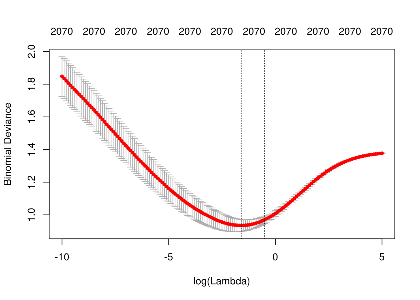

## [1] "Lambda min: 0.201896517994655"
## [1] "Error entrenamiento: 0"
## [1] "Error prueba: 0.21"
## [1] "Devianza entrena:0.261"
## [1] "Devianza prueba:0.879"

No estamos mejorando. Podemos intentar con un número diferente de entradas:

vocabulario <- calc_vocabulario(df_ent, 4000, remove_stop = TRUE)
mod_x <- correr_modelo_cv(df_ent, df_pr, vocabulario, lambda = exp(seq(-10,5,0.1)))
saveRDS(mod_x, file = './cache_obj/mod_sentiment_2.rds')
describir_modelo_cv(mod_x)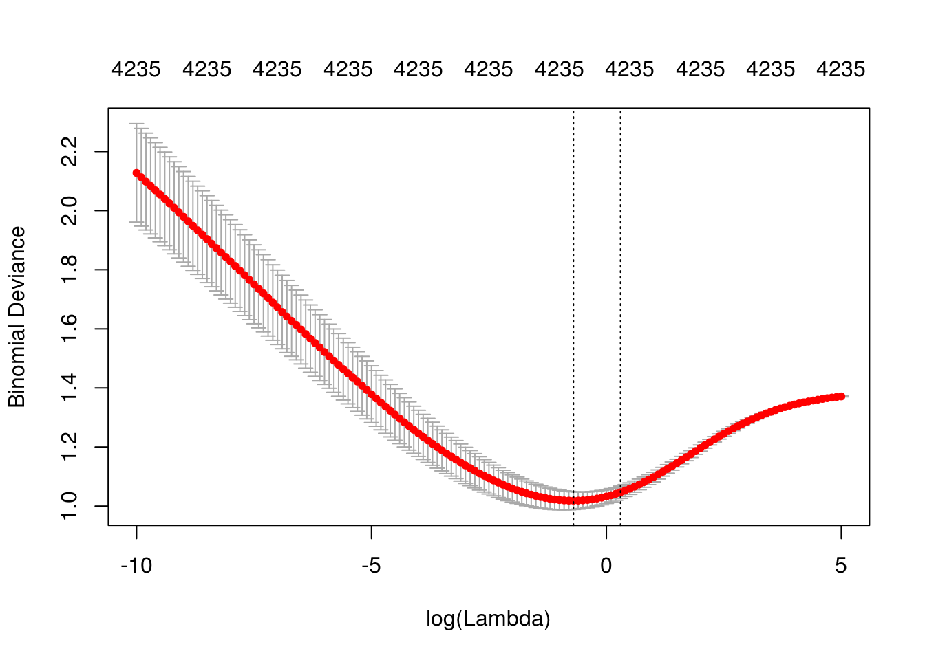

## [1] "Lambda min: 0.49658530379141"
## [1] "Error entrenamiento: 0"
## [1] "Error prueba: 0.18"
## [1] "Devianza entrena:0.295"
## [1] "Devianza prueba:0.883"

Y parece que nuestra estrategia no está funcionando muy bien. Regresamos a nuestro modelo con ridge

vocabulario <- calc_vocabulario(df_ent, 3000, remove_stop = FALSE)
mod_x <- correr_modelo_cv(df_ent, df_pr, vocabulario, lambda = exp(seq(-5,2,0.1)))
saveRDS(mod_x, file = './cache_obj/mod_sentiment_3.rds')
describir_modelo_cv(mod_x)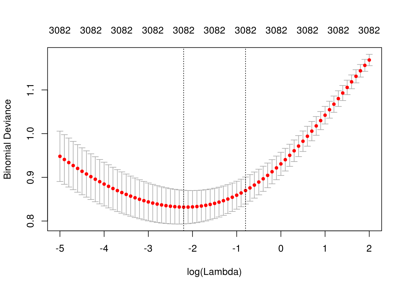

## [1] "Lambda min: 0.110803158362334"
## [1] "Error entrenamiento: 0"
## [1] "Error prueba: 0.18"
## [1] "Devianza entrena:0.128"
## [1] "Devianza prueba:0.775"

Podemos intentar aumentar el número de palabras y aumentar también la regularización

vocabulario <- calc_vocabulario(df_ent, 4000, remove_stop = FALSE)
mod_x <- correr_modelo_cv(df_ent, df_pr, vocabulario, lambda = exp(seq(-5,2,0.1)))
saveRDS(mod_x, file = './cache_obj/mod_sentiment_4.rds')
describir_modelo_cv(mod_x)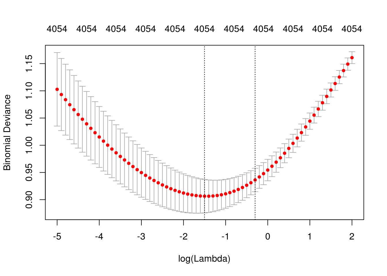

## [1] "Lambda min: 0.22313016014843"
## [1] "Error entrenamiento: 0"
## [1] "Error prueba: 0.16"
## [1] "Devianza entrena:0.173"
## [1] "Devianza prueba:0.776"

6.6 Consiguiendo más datos

Si nuestro problema es varianza, conseguir más datos de entrenamiento puede ayudarnos, especialmente si producir estos datos es relativamente barato y rápido.

Como nuestro principal problema es varianza, podemos mejorar buscando más datos. Supongamos que hacemos eso en este caso, conseguimos el doble casos de entrenamiento. En este ejemplo, podríamos etiquetar más reviews: esto es relativamente barato y rápido

vocabulario <- calc_vocabulario(df_ent_grande, 3000, remove_stop = FALSE)
mod_x <- correr_modelo_cv(df_ent_grande, df_pr, vocabulario, lambda = exp(seq(-5,2,0.1)))

## Joining, by = "palabra"
## Joining, by = "palabra"

## Warning: Trying to compute distinct() for variables not found in the data:
## - `row_col`, `column_col`
## This is an error, but only a warning is raised for compatibility reasons.
## The operation will return the input unchanged.

## Warning: Trying to compute distinct() for variables not found in the data:
## - `row_col`, `column_col`
## This is an error, but only a warning is raised for compatibility reasons.
## The operation will return the input unchanged.

saveRDS(mod_x, file = './cache_obj/mod_sentiment_5.rds')
describir_modelo_cv(mod_x)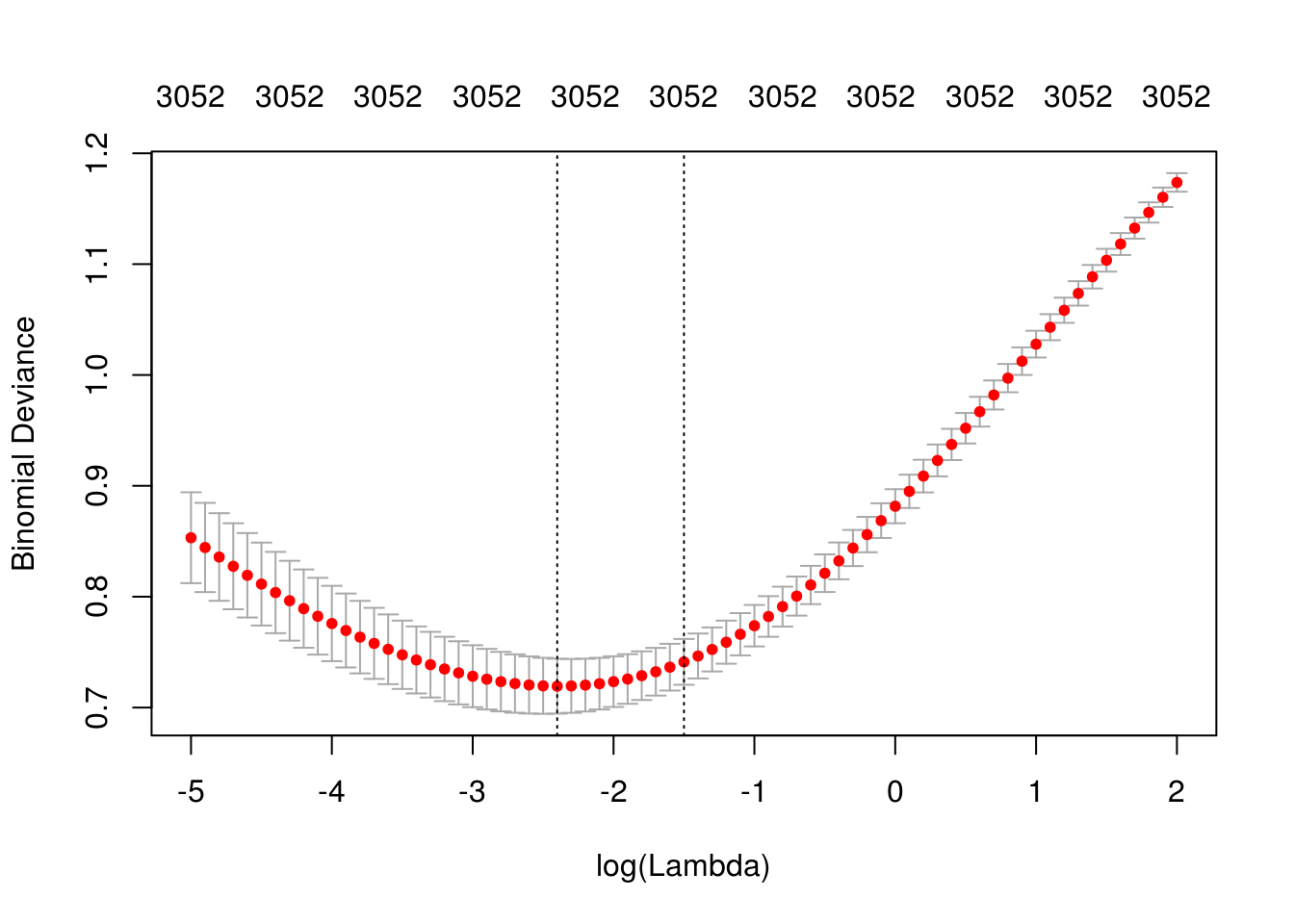

## [1] "Lambda min: 0.0907179532894125"
## [1] "Error entrenamiento: 0"
## [1] "Error prueba: 0.12"
## [1] "Devianza entrena:0.18"
## [1] "Devianza prueba:0.653"

Y ya casi logramos nuestro objetivo. Podemos intentar con más palabras

vocabulario <- calc_vocabulario(df_ent_grande, 4000, remove_stop = FALSE)
mod_x <- correr_modelo_cv(df_ent_grande, df_pr, vocabulario, lambda = exp(seq(-5,2,0.1)))

## Joining, by = "palabra"
## Joining, by = "palabra"

## Warning: Trying to compute distinct() for variables not found in the data:
## - `row_col`, `column_col`
## This is an error, but only a warning is raised for compatibility reasons.
## The operation will return the input unchanged.

## Warning: Trying to compute distinct() for variables not found in the data:
## - `row_col`, `column_col`
## This is an error, but only a warning is raised for compatibility reasons.
## The operation will return the input unchanged.

saveRDS(mod_x, file = './cache_obj/mod_sentiment_6.rds')
mod_x <- readRDS('./cache_obj/mod_sentiment_6.rds')
describir_modelo_cv(mod_x)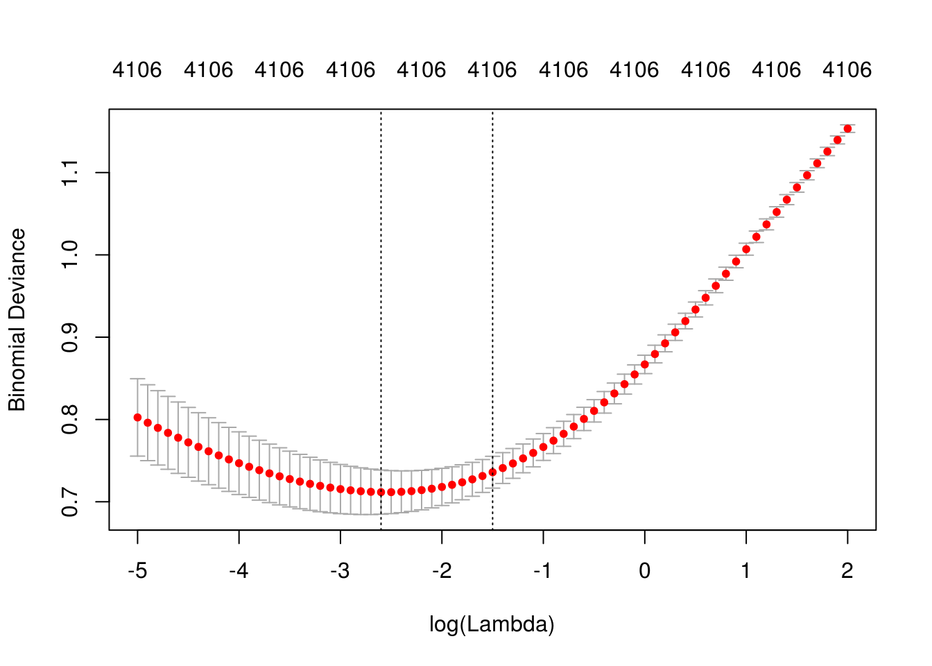

## [1] "Lambda min: 0.0742735782143339"
## [1] "Error entrenamiento: 0"
## [1] "Error prueba: 0.12"
## [1] "Devianza entrena:0.127"
## [1] "Devianza prueba:0.621"

Y esto funcionó bien. Subir más la regularización no ayuda mucho (pruébalo). Parece que el sesgo lo podemos hacer chico (reducir el error de entrenamiento considerablemente), pero tenemos un problema más grande con la varianza.

Quizá muchas palabras que estamos usando no tienen qué ver con la calidad de positivo/negativo, y eso induce varianza.
Estos modelos no utilizan la estructura que hay en las reseñas, simplemente cuentan qué palabras aparecen. Quizá aprovechar esta estructura podemos incluir variables más informativas que induzcan menos varianza sin aumentar el sesgo.
Podemos conseguir más datos.

Obsérvese que:

¿Podríamos intentar con una red neuronal totalmente conexa? Probablemente esto no va a ayudar, pues es un modelo más complejo y nuestro problema es varianza.

6.7 Usar datos adicionales

Considerar fuentes adicionales de datos muchas veces puede ayudar a mejorar nuestras entradas, lo cual puede tener beneficios en predicción (tanto sesgo como varianza).

Intentemos el primer camino. Probamos usar palabras que tengan afinidad como parte de su significado (positivas y negativas). Estos datos están incluidos en el paquete tidytext.

bing <- filter(sentiments, lexicon == 'bing')
tail(bing)

## # A tibble: 6 x 4
##   word      sentiment lexicon score
##   <chr>     <chr>     <chr>   <int>
## 1 zealous   negative  bing       NA
## 2 zealously negative  bing       NA
## 3 zenith    positive  bing       NA
## 4 zest      positive  bing       NA
## 5 zippy     positive  bing       NA
## 6 zombie    negative  bing       NA

dim(vocabulario)

## [1] 4106    2

vocabulario <- calc_vocabulario(df_ent_grande, 8000, remove_stop = FALSE)
voc_bing <- vocabulario %>% inner_join(bing %>% rename(palabra = word))

## Joining, by = "palabra"

dim(voc_bing)

## [1] 1476    5

mod_x <- correr_modelo_cv(df_ent_grande, df_pr, voc_bing, alpha=0,
                       lambda = exp(seq(-5,2,0.1)))

## Joining, by = "palabra"
## Joining, by = "palabra"

## Warning: Trying to compute distinct() for variables not found in the data:
## - `row_col`, `column_col`
## This is an error, but only a warning is raised for compatibility reasons.
## The operation will return the input unchanged.

## Warning: Trying to compute distinct() for variables not found in the data:
## - `row_col`, `column_col`
## This is an error, but only a warning is raised for compatibility reasons.
## The operation will return the input unchanged.

describir_modelo_cv(mod_x)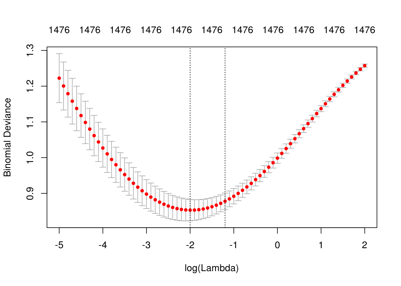

## [1] "Lambda min: 0.135335283236613"
## [1] "Error entrenamiento: 0.02"
## [1] "Error prueba: 0.18"
## [1] "Devianza entrena:0.399"
## [1] "Devianza prueba:0.775"

Estas variables solas no dan un resultado tan bueno (tenemos tanto sesgo como varianza altas). Podemos combinar:

vocabulario <- calc_vocabulario(df_ent_grande, 3000, remove_stop =FALSE)
voc <- bind_rows(vocabulario, voc_bing %>% select(palabra, frec)) %>% unique
dim(voc)

## [1] 4021    2

mod_x <- correr_modelo_cv(df_ent_grande, df_pr, voc, alpha=0, lambda = exp(seq(-5,2,0.1)))

## Joining, by = "palabra"
## Joining, by = "palabra"

## Warning: Trying to compute distinct() for variables not found in the data:
## - `row_col`, `column_col`
## This is an error, but only a warning is raised for compatibility reasons.
## The operation will return the input unchanged.

## Warning: Trying to compute distinct() for variables not found in the data:
## - `row_col`, `column_col`
## This is an error, but only a warning is raised for compatibility reasons.
## The operation will return the input unchanged.

describir_modelo_cv(mod_x)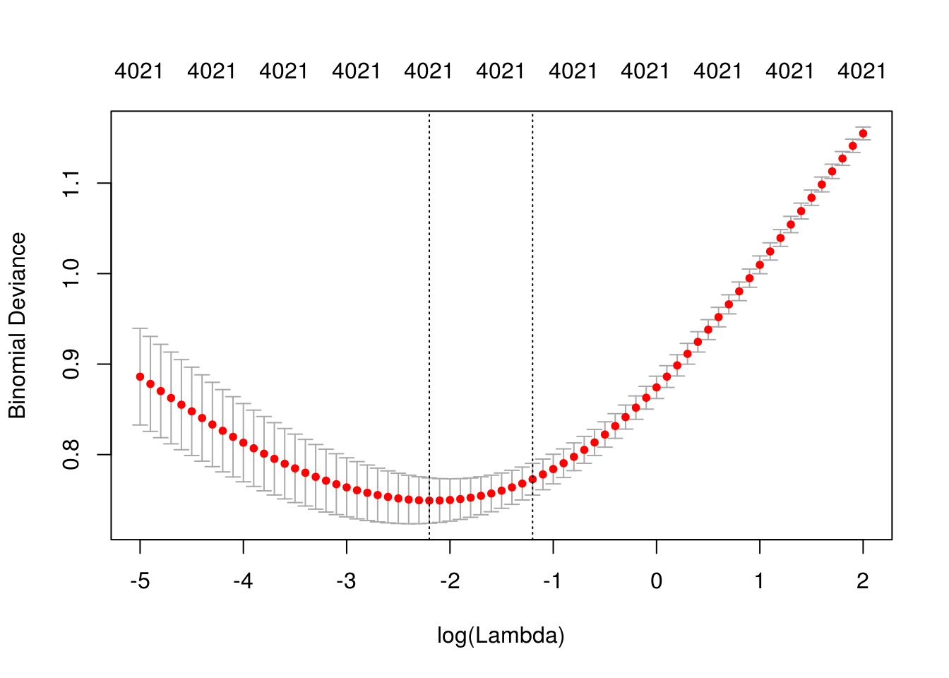

## [1] "Lambda min: 0.110803158362334"
## [1] "Error entrenamiento: 0"
## [1] "Error prueba: 0.13"
## [1] "Devianza entrena:0.168"
## [1] "Devianza prueba:0.64"

Este camino no se ve mal, pero no hemos logrado mejoras. Aunque quizá valdría la pena intentar refinar más y ver qué pasa.

6.8 Examen de modelo y Análisis de errores

Ahora podemos ver qué errores estamos cometiendo, y cómo está funcionando el modelo. Busquemos los peores. Corremos el mejor modelo hasta ahora:

vocabulario <- calc_vocabulario(df_ent_grande, 4000, remove_stop = FALSE)
mod_x <- correr_modelo_cv(df_ent_grande, df_pr, vocabulario, lambda = exp(seq(-5,2,0.1)))

## Joining, by = "palabra"
## Joining, by = "palabra"

## Warning: Trying to compute distinct() for variables not found in the data:
## - `row_col`, `column_col`
## This is an error, but only a warning is raised for compatibility reasons.
## The operation will return the input unchanged.

## Warning: Trying to compute distinct() for variables not found in the data:
## - `row_col`, `column_col`
## This is an error, but only a warning is raised for compatibility reasons.
## The operation will return the input unchanged.

describir_modelo_cv(mod_x)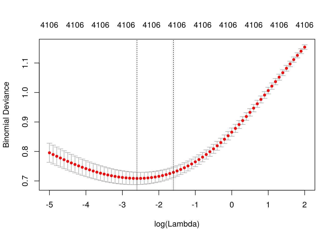

## [1] "Lambda min: 0.0742735782143339"
## [1] "Error entrenamiento: 0"
## [1] "Error prueba: 0.12"
## [1] "Devianza entrena:0.127"
## [1] "Devianza prueba:0.621"

coeficientes <- predict(mod_x$mod, lambda = 'lambda.min', type = 'coefficients') 
coef_df <- data_frame(palabra = rownames(coeficientes),
                      coef = coeficientes[,1])
arrange(coef_df, coef) %>% print(n=20)

## # A tibble: 4,107 x 2
##    palabra        coef
##    <chr>         <dbl>
##  1 (Intercept)  -0.520
##  2 tiresome     -0.318
##  3 sloppy       -0.317
##  4 tedious      -0.313
##  5 designed     -0.287
##  6 profanity    -0.286
##  7 forgot       -0.285
##  8 insulting    -0.273
##  9 redeeming    -0.268
## 10 ludicrous    -0.267
## 11 asleep       -0.264
## 12 embarrassing -0.260
## 13 alas         -0.254
## 14 miserably    -0.252
## 15 lifeless     -0.247
## 16 random       -0.242
## 17 abilities    -0.238
## 18 ridiculous   -0.235
## 19 inept        -0.234
## 20 stupidity    -0.231
## # ... with 4,087 more rows

arrange(coef_df, desc(coef)) %>% print(n=20)

## # A tibble: 4,107 x 2
##    palabra       coef
##    <chr>        <dbl>
##  1 refreshing   0.306
##  2 beings       0.289
##  3 underneath   0.287
##  4 commanding   0.260
##  5 outstanding  0.245
##  6 marvelous    0.236
##  7 finest       0.230
##  8 identify     0.228
##  9 enjoyment    0.228
## 10 ralph        0.224
## 11 exceptional  0.220
## 12 threatens    0.218
## 13 mature       0.216
## 14 anger        0.216
## 15 luckily      0.214
## 16 enters       0.213
## 17 overall      0.210
## 18 breathtaking 0.208
## 19 popcorn      0.207
## 20 portrait     0.205
## # ... with 4,087 more rows

Y busquemos las diferencias más grandes del la probabilidad ajustada con la clase observada

y <- mod_x$prueba$y
x <- mod_x$prueba$x
probs <- predict(mod_x$mod, newx = x, type = 'response', s ='lambda.min')
df_1 <- data_frame(id = rownames(x), y=y, prob = probs[,1]) %>%
  mutate(error = y - prob) %>% arrange(desc(abs(error)))
df_1

## # A tibble: 425 x 4
##    id        y   prob  error
##    <chr> <dbl>  <dbl>  <dbl>
##  1 1508      1 0.0370  0.963
##  2 1461      1 0.0459  0.954
##  3 1490      1 0.0900  0.910
##  4 222       0 0.896  -0.896
##  5 1933      1 0.106   0.894
##  6 1642      1 0.131   0.869
##  7 25        0 0.864  -0.864
##  8 728       0 0.860  -0.860
##  9 1050      1 0.146   0.854
## 10 415       0 0.850  -0.850
## # ... with 415 more rows

filter(df_pr, id == 1461) %>% pull(texto) %>% str_sub(1, 500)

[1] “Review deep rising is one of " those " movies . the kind of movie which serves no purpose except to entertain us . it does not ask us to think about important questions like life on other planets or the possibility that there is no god . . . screw that , it says boldly , let’s see some computer generated monsters rip into , decapitate and generally cause irreparable booboos to a bunch of little known actors . heh ! them wacky monsters , gotta love ’em . of course , since we can rent about”

filter(df_pr, id == 1508) %>% pull(texto) %>% str_sub(1, 1000)

[1] “Review capsule : side-splitting comedy that follows its own merciless logic almost through to the end . . . but not without providing a good deal of genuine laughs . most comedies these days have one flaw . they’re not funny . they think they’re funny , but they are devoid of anything really penetrating or dastardly . occasionally a good funny movie sneaks past the deadening hollywood preconceptions of humor and we get a real gem : ruthless people , for instance , which established a microcosm of a setup and played it out to the bitter end . liar liar is built the same way and is just about as funny . this is one of the few movies i’ve seen where i was laughing consistently almost all the way through : instead of a couple of set-pieces that inspired a laugh ( think of the dismal fatal instinct ) , the whole movie works like clockwork . jim carrey playes a high-powered lawyer , to whom lying is as natural as breathing . there is one thing he takes seriously , though : his son”

Estas últimas son reseñas positivas que clasificamos incorrectamente como negativas. Vemos que en ambas el tono es irónico: por ejemplo, la primera argumenta que la película es mala, pero disfrutable. Esta fue etiquetada como una reseña positiva.

Este fenómeno se puede ver como un problema difícil de sesgo: nuestro modelo simple difícilmente podrá captar esta estructura compleja de ironía.

El problema es diferente para las reseñas negativas. Veamos algunas de las reseñas negativas peor clasificadas:

filter(df_pr, id == 222) %>% pull(texto) %>% str_sub(1, 1000) #negativa

[1] “Review it’s probably inevitable that the popular virtual reality genre ( " the matrix , " " existenz " ) would collide with the even more popular serial-killer genre ( " kiss the girls , " " se7en " ) . the result should have been more interesting than " the cell . " as the movie opens , therapist catharine deane ( jennifer lopez ) treats a catatonic boy ( colton james ) by entering his mind through some sort of virtual reality technique that’s never fully explained . after months of therapy sessions in a surreal desert , catharine has no success to report . meanwhile , killer carl stargher ( vincent d’onofrio ) has claimed another victim . his particular hobby is to kidnap young women , keep them in a glass cell overnight , and drown them . he takes the corpse and soaks it in bleach , then suspends himself over the body and jerks off while watching a video tape of the drowning . although carl’s been doing this for awhile , he’s recently become sloppy , and fbi agent peter nova”

filter(df_pr, id == 728) %>% pull(texto) %>% str_sub(1, 1000) #negativa

[1] “Review girl 6 is , in a word , a mess . i was never able to determine what spike lee was trying to accomplish with this film . there was no sense of where the film was going , or any kind of coherent narrative . if there was a point to the film , i missed it . girl 6 , by the way , is the way theresa randle’s character is addressed in the phone sex workplace ; all the girls are known by their numbers . the plot , such as it is : theresa randle is a struggling n . y . actress , and eventually takes a job as a phone-sex operator . she begins to lose contact with reality , as her job consumes her . also , she must deal with the advances of her ex-husband ( isiah washington ) . he is an ex- con thief , and she tries to keep him away , while at the same time , it’s clear that she still harbors feelings for him . her neighbor , jimmy ( spike lee ) functions as the observer ; mediating between the ex- husband and girl 6 . he also functions as a point of stability , as he watches he”

No está totalmente claro por qué nos equivocamos en estas dos reseñas. Podemos hacer un examen más cuidadoso de la construcción del predictor, obteniendo los coeficientes \(\beta\) y el vector \(x\) con los que se construyen el predictor:

beta <- coef(mod_x$mod) %>% as.numeric
nombres <- rownames(x)
head(sort(x[nombres == "222", ], decreasing = TRUE), 100)

##       the        in        of        to         a       and        is 
##        52        21        17        17        16        14        10 
##      cell      mind      have      that      this        as      been 
##         9         7         5         5         5         4         4 
##       has       his     horse    killer      more       she      than 
##         4         4         4         4         4         4         4 
##      with       all        an   another        by     could      fast 
##         4         3         3         3         3         3         3 
##       for     glass       out     peter     seems    should     video 
##         3         3         3         3         3         3         3 
##     after        at    before       boy       can  computer developed 
##         2         2         2         2         2         2         2 
##      find      from generated     genre        go        he       him 
##         2         2         2         2         2         2         2 
##         i      into        it      it's      keep      like     movie 
##         2         2         2         2         2         2         2 
##        no       not       off        on       one        or       own 
##         2         2         2         2         2         2         2 
##   popular   promise   reality    really      room   surreal      them 
##         2         2         2         2         2         2         2 
##      time  universe   virtual      well    acting     agent  although 
##         2         2         2         2         1         1         1 
##     apart    attack        be   because    become     begin      best 
##         1         1         1         1         1         1         1 
##   bizarre      body    bottom    brings       but     catch    center 
##         1         1         1         1         1         1         1 
## character   closing  costumes   creates      dark  darkness       day 
##         1         1         1         1         1         1         1 
##     depth    desert 
##         1         1

predictor <- beta * c(1, x[nombres=="222",])  # beta*x
sum(predictor)

## [1] 1.437326

sort(predictor[predictor != 0]) %>% knitr::kable()

	x
	-0.5202993
sloppy	-0.3172574
promise	-0.2760900
video	-0.1501897
dull	-0.1331210
catch	-0.1169287
should	-0.1159415
suffers	-0.1128175
trapped	-0.1111792
could	-0.1011409
pulling	-0.1003304
bottom	-0.0939438
fast	-0.0911754
been	-0.0908088
save	-0.0876571
explained	-0.0808605
have	-0.0796675
mtv	-0.0714969
talking	-0.0639503
kidnapped	-0.0600789
water	-0.0600346
vince	-0.0571824
begin	-0.0547786
jennifer	-0.0528719
virtual	-0.0519579
twisted	-0.0508402
center	-0.0505813
provided	-0.0492090
psycho	-0.0489186
off	-0.0482361
recently	-0.0482342
result	-0.0476513
women	-0.0472648
point	-0.0472133
within	-0.0458799
forward	-0.0456438
exercise	-0.0452252
no	-0.0410514
technique	-0.0405685
director	-0.0358213
focus	-0.0351205
acting	-0.0345010
interesting	-0.0334681
style	-0.0332168
thomas	-0.0322831
kept	-0.0316398
hardly	-0.0309470
another	-0.0307244
attack	-0.0302758
explored	-0.0292849
then	-0.0292602
or	-0.0290317
victim	-0.0276020
fill	-0.0267911
hope	-0.0266701
even	-0.0250174
enough	-0.0249711
woman	-0.0244227
fall	-0.0234435
apart	-0.0233941
out	-0.0230786
this	-0.0196350
to	-0.0184586
premise	-0.0180929
she’s	-0.0179955
killer	-0.0173511
left	-0.0173469
development	-0.0172162
how	-0.0165661
into	-0.0162641
at	-0.0153004
discover	-0.0150697
them	-0.0133533
would	-0.0129188
james	-0.0124600
on	-0.0124260
where	-0.0121713
sort	-0.0121419
much	-0.0114857
costumes	-0.0111567
turns	-0.0110439
so	-0.0108164
movie	-0.0108057
end	-0.0107060
review	-0.0105867
be	-0.0104210
don’t	-0.0102111
had	-0.0100659
like	-0.0100186
because	-0.0099953
seems	-0.0096492
girls	-0.0096262
tape	-0.0089222
through	-0.0089024
character	-0.0087373
all	-0.0081031
room	-0.0078808
long	-0.0074416
get	-0.0068225
some	-0.0054598
thought	-0.0052326
fbi	-0.0052078
bizarre	-0.0050159
opportunity	-0.0048392
house	-0.0047232
forty	-0.0037017
after	-0.0036686
minds	-0.0035547
doing	-0.0035518
my	-0.0030584
hours	-0.0030343
scene	-0.0029061
girl	-0.0026162
i	-0.0024423
psychotic	-0.0014919
next	-0.0013199
singer	-0.0012470
that	-0.0007843
watching	-0.0000763
but	0.0001236
standing	0.0002228
himself	0.0003255
pieces	0.0003999
popular	0.0007742
its	0.0017265
she	0.0022264
can	0.0025564
think	0.0025935
they	0.0027960
over	0.0029586
part	0.0036062
personality	0.0037015
he’s	0.0039892
one	0.0040252
existenz	0.0040481
never	0.0042116
it	0.0042247
substance	0.0042565
that’s	0.0045095
kiss	0.0054557
an	0.0056231
known	0.0057068
really	0.0057512
element	0.0058064
not	0.0059663
place	0.0060158
horse	0.0070165
go	0.0072319
without	0.0073540
time	0.0078486
however	0.0078614
for	0.0081780
their	0.0088714
first	0.0093176
closing	0.0100908
serial	0.0104635
of	0.0108933
rather	0.0113546
opens	0.0114884
him	0.0115767
michael	0.0115885
he	0.0116202
living	0.0126425
fate	0.0126835
meanwhile	0.0129676
though	0.0129746
his	0.0136937
slow	0.0141722
peter	0.0144512
vincent	0.0148222
young	0.0150035
day	0.0150646
does	0.0152965
it’s	0.0154444
by	0.0156547
depth	0.0156696
importance	0.0159429
while	0.0163877
will	0.0164211
world	0.0165024
has	0.0168118
particular	0.0174925
more	0.0176460
a	0.0189342
effect	0.0193250
agent	0.0199253
creates	0.0209483
leaves	0.0215036
see	0.0217573
with	0.0231662
role	0.0232334
from	0.0234281
body	0.0234823
than	0.0237709
probably	0.0239042
developed	0.0240430
elaborate	0.0243947
suddenly	0.0247735
logic	0.0249532
most	0.0265502
line	0.0271946
music	0.0273477
as	0.0278241
still	0.0292254
months	0.0294009
shows	0.0296746
psychological	0.0313499
head	0.0321303
boy	0.0340266
darkness	0.0342972
become	0.0346070
very	0.0348716
father	0.0352316
although	0.0354252
sound	0.0358830
finds	0.0375483
matrix	0.0377628
particularly	0.0390302
brings	0.0400255
success	0.0403674
before	0.0412008
directing	0.0413102
viewer	0.0421106
sidney	0.0425819
best	0.0432040
the	0.0439582
is	0.0443391
takes	0.0448486
dark	0.0449853
inside	0.0476245
separate	0.0479765
in	0.0487678
find	0.0500643
great	0.0523020
together	0.0581238
computer	0.0586483
genre	0.0593194
own	0.0625957
reality	0.0627538
disturbing	0.0636809
keep	0.0642032
and	0.0648463
offer	0.0736850
strangely	0.0743557
inevitable	0.0759366
fully	0.0789776
jake	0.0797114
frightened	0.0824091
provoking	0.0846733
well	0.0880060
desert	0.0899893
treats	0.0985579
losing	0.0990976
religion	0.1298072
generated	0.1304031
universe	0.1438618
madness	0.1580777
sharp	0.1604157
enters	0.2131698
surreal	0.2394179
mind	0.2858087
glass	0.4687988
cell	0.7086423

beta <- coef(mod_x$mod) %>% as.numeric
nombres <- rownames(x)
predictor <- beta * c(1, x[nombres=="728",])  # beta*x
sum(predictor)

## [1] 1.177288

sort(predictor[predictor != 0]) %>% knitr::kable()

	x
	-0.5202993
mess	-0.2022808
impression	-0.1506333
grade	-0.1503932
struggling	-0.1301878
there	-0.1228140
loud	-0.1042231
point	-0.0944266
onscreen	-0.0910190
nothing	-0.0838901
tries	-0.0810926
stuck	-0.0777950
seemed	-0.0768979
numbers	-0.0716475
bad	-0.0704995
confused	-0.0645791
con	-0.0619718
missed	-0.0598450
sex	-0.0582862
wasn’t	-0.0534325
even	-0.0500348
phone	-0.0499893
plot	-0.0488645
women	-0.0472648
lose	-0.0471523
stone	-0.0467291
middle	-0.0416681
lee	-0.0414526
trying	-0.0402636
should	-0.0386472
was	-0.0380697
any	-0.0374969
sequences	-0.0373245
only	-0.0365272
buddy	-0.0357364
he’d	-0.0345297
acting	-0.0345010
interesting	-0.0334681
i’d	-0.0325935
kept	-0.0316398
be	-0.0312630
if	-0.0309857
fan	-0.0303648
becomes	-0.0292044
or	-0.0290317
idea	-0.0261244
die	-0.0243408
such	-0.0222690
i’m	-0.0215163
actress	-0.0205609
no	-0.0205257
hard	-0.0196748
character	-0.0174746
some	-0.0163793
away	-0.0162291
have	-0.0159335
girl	-0.0156973
happens	-0.0150229
make	-0.0141744
to	-0.0130296
background	-0.0129527
where	-0.0121713
this	-0.0117810
setup	-0.0115887
much	-0.0114857
d	-0.0113921
made	-0.0112626
gave	-0.0109618
going	-0.0106231
might	-0.0105983
review	-0.0105867
scenes	-0.0100794
had	-0.0100659
like	-0.0100186
later	-0.0097639
girls	-0.0096262
up	-0.0090409
course	-0.0089834
just	-0.0083408
her	-0.0082487
into	-0.0081321
out	-0.0076929
at	-0.0076502
jimmy	-0.0071043
when	-0.0057891
work	-0.0054795
seems	-0.0032164
my	-0.0030584
thing	-0.0029429
scene	-0.0029061
all	-0.0027010
i	-0.0024423
that	-0.0015686
altogether	-0.0006508
opening	0.0001563
but	0.0002473
amusing	0.0003099
songs	0.0007721
fans	0.0014369
which	0.0015447
she	0.0022264
begins	0.0022827
really	0.0028756
past	0.0029292
an	0.0037487
time	0.0039243
more	0.0044115
are	0.0047948
ex	0.0049676
they	0.0055921
me	0.0057067
known	0.0057068
than	0.0059427
not	0.0059663
one	0.0060378
who	0.0067409
other	0.0076092
it’s	0.0077222
however	0.0078614
types	0.0080658
for	0.0081780
same	0.0082892
has	0.0084059
determine	0.0084183
never	0.0084232
sense	0.0084978
thief	0.0094086
it	0.0105618
of	0.0108933
rather	0.0113546
him	0.0115767
grows	0.0122519
sequence	0.0122732
dollar	0.0123269
love	0.0130239
a	0.0142007
kind	0.0150748
use	0.0150783
lives	0.0152753
you	0.0153545
must	0.0160841
what	0.0161985
while	0.0163877
will	0.0164211
world	0.0165024
their	0.0177427
feelings	0.0178434
word	0.0180196
washington	0.0198875
grant	0.0199556
by	0.0208729
parts	0.0210454
prince	0.0216244
taking	0.0221986
with	0.0231662
from	0.0234281
probably	0.0239042
way	0.0242771
i’ve	0.0245634
worked	0.0249386
in	0.0255450
few	0.0262726
done	0.0263053
the	0.0287419
n	0.0287966
still	0.0292254
biggest	0.0296875
is	0.0310374
reality	0.0313769
keep	0.0321016
good	0.0340647
film	0.0344213
always	0.0348183
very	0.0348716
and	0.0370550
moments	0.0371737
between	0.0372559
though	0.0389237
particularly	0.0390302
agree	0.0441769
takes	0.0448486
able	0.0480575
i’ll	0.0480974
eventually	0.0484890
born	0.0494355
shot	0.0500720
different	0.0507236
several	0.0510954
he	0.0522909
killers	0.0530381
clear	0.0549046
attention	0.0549228
contact	0.0574982
as	0.0626043
multi	0.0640192
deal	0.0648396
also	0.0659141
become	0.0692140
fairly	0.0745365
narrative	0.0791347
performances	0.0816109
music	0.0820430
neighbor	0.0848025
watches	0.0876229
broke	0.0936433
natural	0.0969546
reminiscent	0.1004395
voices	0.1151647
excellent	0.1228298
intense	0.1262374
frightening	0.1264323
oliver	0.1275805
job	0.1327543
husband	0.1379187
distracting	0.1526334
soundtrack	0.1612572
industry	0.2074668
6	0.4226458

Y notamos que en primer caso, palabras “cell” es consideradas como positivas y en el segundo caso, se considera la ocurrencia de “6” como positiva. Sin embargo, observamos que en ambos casos la palabra problemática es usada de manera distinta en estas reseñas que en el resto (la primera es la película The Cell, y la segunda es Girl 6). La frecuencia alta de estas palabras en estas dos reseñas contribuye incorrectamente a denotar estas reseñas como positivas.

Estas películas extrapolan demasiado lejos de los datos de entrenamiento. Típicamente, la extrapolación fuerte produce problemas tanto de sesgo (modelo poco apropiado para los valores que observamos) como varianza, pues estamos haciendo predicciones donde hay pocos datos.

En este caso, podemos intentar reducir el sesgo tomando el logaritmo de los conteos de palabras en lugar de los conteos crudos. Esto reduce la influencia de conteos altos de palabras en relación a conteos altos (también podemos intentar usar indicadoras 0-1 en lugar de conteos). Después de algunos experimentos, podemos mejorar un poco:

usar_cache <- TRUE
vocabulario <- calc_vocabulario(df_ent_grande, 8500, remove_stop = FALSE)
if(!usar_cache){
    mod_x <- correr_modelo_cv(df_ent_grande, df_pr, vocabulario, 
                              alpha = 0.01, lambda = exp(seq(-5, 2, 0.1)),
                              log_transform = TRUE)
    saveRDS(mod_x, file = "./cache_obj/mod_sentiment_log.rds")
  } else {
    mod_x <- readRDS("./cache_obj/mod_sentiment_log.rds")
  }
describir_modelo_cv(mod_x)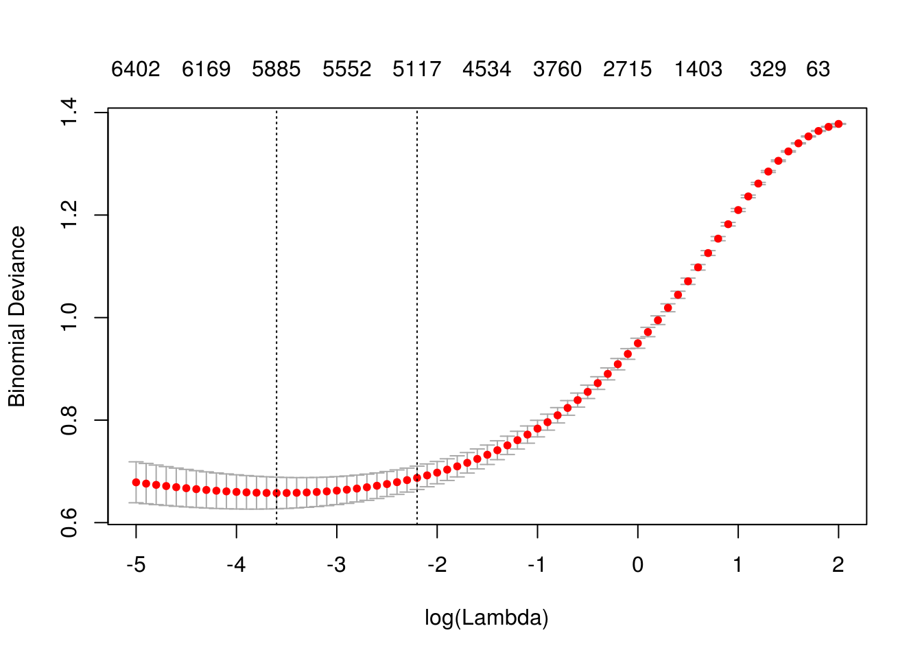

## [1] "Lambda min: 0.0273237224472926"
## [1] "Error entrenamiento: 0"
## [1] "Error prueba: 0.11"
## [1] "Devianza entrena:0.045"
## [1] "Devianza prueba:0.565"